How to Remove Invisible Characters in Excel: Banish VLOOKUP Errors and Data Frustration Forever!

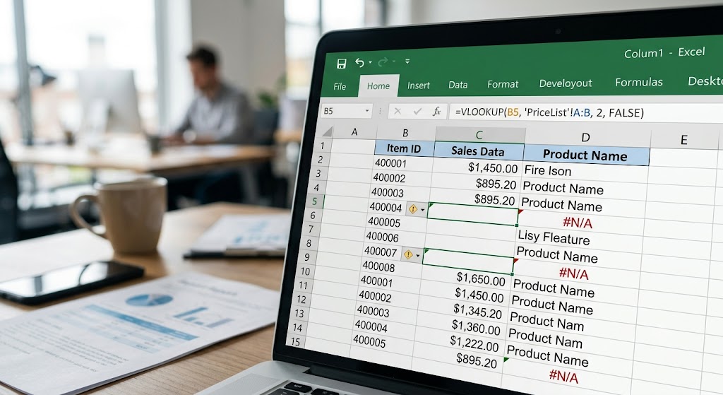
Ah, the classic office worker dilemma. You’re racing against a deadline, piecing together crucial reports, and Excel is your trusty steed. You confidently enter your VLOOKUP formula, hit Enter, and… #N/A. Or worse, the numbers just don’t add up, filters don’t work, and data that *looks* identical refuses to match. You stare at the screen, baffled, convinced Excel is playing a cruel joke. Sound familiar?

You’re not alone. This infuriating scenario is a daily battle for countless professionals, and the silent saboteurs behind it are often invisible characters in Excel. These rogue, non-printing characters hide in plain sight, causing everything from minor annoyances to major data integrity headaches. They’re the reason your perfectly typed VLOOKUP fails, why a simple COUNTIF returns zero, or why sorting goes awry.

But fear not, fellow data warrior! This comprehensive guide will equip you with the knowledge and tools to identify and remove invisible characters in Excel, transforming your spreadsheets from battlegrounds of frustration into fields of pristine, workable data. We’ll dive deep into using Excel’s powerful CLEAN and TRIM functions, alongside the versatile FIND & REPLACE feature, to reclaim your data sanity.

The Silent Saboteurs: What Are Invisible Characters?

So, what exactly are these elusive characters? Invisible characters are non-printing characters that Excel, and other software, interpret as data, even though they don’t appear visually on your screen. They often find their way into your spreadsheets when you:

• Copy and paste data from websites, PDFs, or other documents.
• Import data from databases or external systems.
• Receive files from colleagues who might have inadvertently introduced them.

Common culprits include:

• Extra Spaces: Leading spaces, trailing spaces, or multiple spaces between words.
• Line Feeds (CHAR(10)): Used for new lines within a cell (often entered with Alt+Enter).
• Carriage Returns (CHAR(13)): Similar to line feeds, another form of line break.
• Non-Breaking Spaces (CHAR(160)): Often found when pasting from web pages, these look like regular spaces but are distinct characters.
• Other Non-Printable Characters: A range of control characters (ASCII values 0-31) that might be used for formatting or system commands but are useless, or harmful, in your data.

These seemingly innocuous characters create discrepancies that Excel’s functions, like VLOOKUP, cannot overlook. To Excel, “Apple” and ” Apple” (with a leading space) are completely different values. This is why knowing how to remove invisible characters excel data becomes crucial.

Detecting the Undetectable: How to Spot Invisible Characters

While their nature is to be invisible, you can often get clues:

• Unexpected Cell Length: Use the LEN() function. If =LEN(A2) returns 6 for “Apple”, but =LEN(B2) returns 7 for a cell that also *looks* like “Apple”, you likely have an invisible character in B2.
• VLOOKUP/MATCH Errors: As we discussed, these are the classic tell-tale signs.
• Filter/Sort Anomalies: Data that should group together doesn’t, or sorts incorrectly.

But why just detect when you can eliminate? Let’s get to the practical solutions to remove invisible characters excel style!

Method 1: The Dynamic Duo – CLEAN and TRIM Functions

Excel’s CLEAN and TRIM functions are your first line of defense against most common invisible character issues. They are incredibly powerful, especially when used in combination.

1. The CLEAN Function

The CLEAN function is designed to remove all non-printable characters from text. These are typically the first 32 non-printing characters in the 7-bit ASCII code (values 0 through 31). This includes characters like line breaks (CHAR(10) and CHAR(13)) that often plague imported data.

• Syntax: =CLEAN(text)
• Example: If cell A2 contains “Product Name” with a hidden line break, =CLEAN(A2) will return “Product Name” without the line break.

2. The TRIM Function

The TRIM function specializes in removing extra spaces from text. Specifically, it removes:

• All leading spaces (spaces at the beginning of the text).
• All trailing spaces (spaces at the end of the text).
• Reduces multiple spaces between words to a single space.

It does *not* remove non-breaking spaces (CHAR(160)) or other non-printable characters like line breaks.

• Syntax: =TRIM(text)
• Example: If cell A2 contains ” Product Name ” (with leading/trailing spaces), =TRIM(A2) will return “Product Name”. If A2 contains “Product Name” (with multiple spaces), it returns “Product Name”.

3. Using CLEAN and TRIM Together for Maximum Impact

Since CLEAN handles non-printable characters and TRIM handles spaces, combining them is often the most robust solution to remove invisible characters in Excel. Imagine you have data copied from a web page that includes both line breaks and extraneous spaces.

Steps to Apply CLEAN and TRIM:

1. Insert a Helper Column: Let’s say your messy data is in column A, starting from A2. Insert a new column next to it (e.g., column B).
2. Apply the Combined Formula: In cell B2, enter the formula: =TRIM(CLEAN(A2)).
3. Drag Down: Drag the fill handle (the small square at the bottom-right of B2) down to apply the formula to all relevant cells in column B.
4. Copy and Paste as Values:
   • Select all the cells in your helper column (B2 onwards).
   • Copy them (Ctrl+C).
   • Select the original column (A2 onwards) where you want the cleaned data.
   • Right-click and choose Paste Special > Values (or use the shortcut Alt+E, S, V, Enter). This replaces the original messy data with its clean, static value.
5. Delete the Helper Column: Once confirmed, you can delete the helper column.

This powerful combination will significantly improve your data quality and eliminate those pesky VLOOKUP errors by effectively cleaning up most common excel invisible characters.

Method 2: The Precision Strike – FIND & REPLACE

While CLEAN and TRIM are fantastic general-purpose tools, sometimes you need a more targeted approach, especially for specific invisible characters like non-breaking spaces (CHAR(160)) or when you want to remove all occurrences of a particular character without creating a helper column.

1. Removing Line Breaks with FIND & REPLACE (The CTRL+J Trick)

This is a lifesaver for data containing accidental (or intentional) line breaks within cells.

1. Select Your Data: Highlight the range of cells you want to clean.
2. Open FIND & REPLACE: Press Ctrl+H to open the Find and Replace dialog box.
3. Find What: Click in the “Find what:” field. Now, hold down the Ctrl key and press J (release both). You won’t see anything, but a small blinking dot or line might appear. This signifies the line break character.
4. Replace With:
   • To remove the line breaks entirely, leave the “Replace with:” field blank.
   • To replace them with a single space (often preferred to avoid merging words), type a single space into the “Replace with:” field.
5. Execute: Click “Replace All”. Excel will tell you how many replacements were made.

This is an incredibly efficient way to remove invisible characters excel users often struggle with, specifically line breaks.

2. Removing Non-Breaking Spaces (CHAR(160)) with FIND & REPLACE

Non-breaking spaces look identical to regular spaces but are different characters (ASCII code 160). TRIM does *not* remove them, which makes them a frequent cause of VLOOKUP failures after you’ve already “cleaned” your data. Here’s how to tackle them:

Option A: Copy the Character

1. Identify a Cell: Find a cell you suspect contains a non-breaking space.
2. Copy the Character: Go into the formula bar (or double-click the cell) and carefully select *just* the suspected non-breaking space, then copy it (Ctrl+C).
3. Open FIND & REPLACE: Select your data range and press Ctrl+H.
4. Paste into Find What: Paste the copied character into the “Find what:” field (Ctrl+V).
5. Replace With: Enter a single regular space (or leave blank if you want to remove it entirely).
6. Execute: Click “Replace All”.

Option B: Using CHAR(160) in a Helper Column (if Find & Replace isn’t working directly)

Sometimes, directly copying the character into Find & Replace can be tricky. A reliable alternative is to use the SUBSTITUTE function with CHAR(160):

1. Insert a Helper Column: Next to your messy data (e.g., column A).
2. Apply the Formula: In cell B2, enter =SUBSTITUTE(A2,CHAR(160)," "). This replaces all non-breaking spaces with regular spaces.
3. Combine with CLEAN/TRIM: For ultimate cleanliness, you might use =TRIM(CLEAN(SUBSTITUTE(A2,CHAR(160)," "))).
4. Copy and Paste as Values: As explained in Method 1, copy your helper column and paste as values over the original data.

Pro Tips for Data Hygiene

• Work on a Copy: Always make a duplicate of your worksheet or workbook before performing extensive data cleaning. This provides a safety net.
• Combine Methods: For the most robust cleaning, consider a multi-pronged attack. Start with a combined TRIM(CLEAN()) formula, then follow up with FIND & REPLACE for specific characters like non-breaking spaces or line breaks that might have been missed or if you want to replace them with something specific.
• Regular Checks: Get into the habit of running a quick LEN() check or testing a small VLOOKUP on new data imports to catch invisible characters early.
• Understand Your Source: If you repeatedly get data with specific invisible characters, try to understand the source and see if they can be prevented upstream.

Conclusion

No more pulling your hair out over baffling VLOOKUP errors! By understanding the menace of invisible characters in Excel and mastering the use of the CLEAN and TRIM functions alongside targeted FIND & REPLACE techniques, you can transform your data cleansing process from a headache into a streamlined operation. You now possess the powerful tools to effectively remove invisible characters excel spreadsheets harbor, ensuring your data is accurate, consistent, and ready for any analysis. Go forth and conquer your spreadsheets, data warrior!